POL 304: Using Data to Understand Politics and Society

class: center, middle, inverse, title-slide

.title[
# POL 304: Using Data to Understand Politics and Society
]
.subtitle[
## Regression Discontinuity Design
]
.author[
### Olga Chyzh [www.olgachyzh.com]
]

---

## Regression Discontinuity Design

- So far, we said that we can interpret the difference in the outcome between the treatment and the control group as the causal effect of the treatment, as long as there are no confounders (the groups are the same on all variables other than the treatment).

- This is achieved by random assignment.

- In observational data, treatment is not randomly assigned--there are many possible confounders.

- We have discussed several research designs to address this problem.

- RD is another natural experiment design that helps account for confounders.

---
## Example: Does Holding Office Increase Personal Wealth?

- Cannot simply compare people who held office with those who did not. Why?

- Data on political candidates' wealth at the time of death.

- Subset data just to the close elections (Why?)

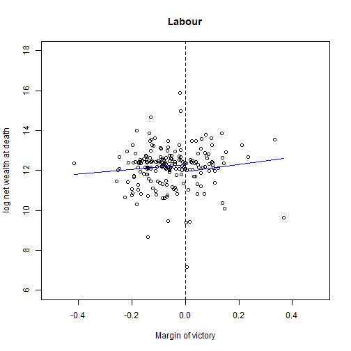
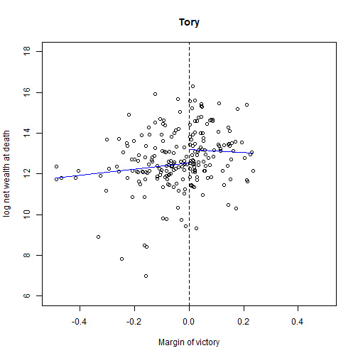
- Regress wealth on the electoral margin, separately for winners and losers (2 regressions).

---

## Does Holding Office Increase Personal Wealth?

---
## Causal Effect for Tory
<img src="06_discontinuity_design_files/figure-html/unnamed-chunk-2-1.png" width="500px" style="display: block; margin: auto;" />

---
## Average Net Wealth for Tory MP

```r
## 
tory.fit1<-lm(ln.net ~ margin, data = MPs.tory[MPs.tory$margin > 0, ])
coef(tory.fit1)
```

```
## (Intercept)      margin 
##   13.187802   -0.727782
```

```r
exp(13.1878)
```

```
## [1] 533812.5
```

---
## Average Net Wealth for Tory Non-MP

```r
tory.fit0<-lm(ln.net ~ margin, data = MPs.tory[MPs.tory$margin < 0, ])
coef(tory.fit0)
```

```
## (Intercept)      margin 
##   12.538116    1.491119
```

```r
exp(12.538)
```

```
## [1] 278730.3
```
---
## Causal Effect

```r
exp(13.1878) - exp(12.538)
```

```
## [1] 255082.2
```

---
## Assumption Check

- Is the treatment assignment (whether a candidate wins or loses by a small margin) truly random?  If some candidates win systematically (e.g., election fraud), then this assumption is violated.

- One way to check is to see if there is a correlation in the margin of victory from one election to the next.

```r
## two regressions for Tory: negative and positive margin
tory.fit3 <- lm(margin.pre ~ margin, data = MPs.tory[MPs.tory$margin < 0, ])
tory.fit4 <- lm(margin.pre ~ margin, data = MPs.tory[MPs.tory$margin > 0, ])
## the difference between two intercepts is the estimated effect
coef(tory.fit4)[1] - coef(tory.fit3)[1]
```

```
## (Intercept) 
## -0.01725578
```

- Small difference, so can assume that the treatment is as-if random.

---
## Example: Government Funding and Literacy Rate

- Litschig, Stephan, and Kevin M Morrison. 2013. “[The Impact of Intergovernmental Transfers on Education Outcomes and Poverty Reduction.](http://dx.doi.org/10.1257/app.5.4.206)” *American Economic Journal: Applied Economics* 5(4): 206–40.

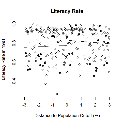
- Discontinuity: discrete thresholds (population cut-offs) in funding allocation (10,188, 13,584, and 16,980)

- Idea: a city of 10,187 people is not any different than that of 10,189 people, yet the latter received significantly more funding.

---
## Government Funding and Literacy Rate

---
## Causal Effect of Funding

```r
lm(literate91 ~ pscore, data = dta.below)
```

```
## 
## Call:
## lm(formula = literate91 ~ pscore, data = dta.below)
## 
## Coefficients:
## (Intercept)       pscore  
##    0.775610     0.006948
```

```r
lm(literate91 ~ pscore, data = dta.above)
```

```
## 
## Call:
## lm(formula = literate91 ~ pscore, data = dta.above)
## 
## Coefficients:
## (Intercept)       pscore  
##      0.8313      -0.0126
```

```r
0.8313-0.775610
```

```
## [1] 0.05569
```

---
## Other Discontinuities

- Can you think of other examples of discontinuities?

---
## Beware!

---
class: inverse, middle, center
# Lab
---

## Does Holding Office Increase Personal Wealth?

```r
## load the data and subset them into two parties
MPs <- read.csv("data/MPs.csv")
MPs.labour <- subset(MPs, subset = (party == "labour"))
MPs.tory <- subset(MPs, subset = (party == "tory"))

## two regressions for Labour: negative and positive margin
labour.fit1 <- lm(ln.net ~ margin,
                  data = MPs.labour[MPs.labour$margin < 0, ])
labour.fit2 <- lm(ln.net ~ margin,
                  data = MPs.labour[MPs.labour$margin > 0, ])

## two regressions for Tory: negative and positive margin
tory.fit1 <- lm(ln.net ~ margin, data = MPs.tory[MPs.tory$margin < 0, ])
tory.fit2 <- lm(ln.net ~ margin, data = MPs.tory[MPs.tory$margin > 0, ])
```

---
## Make a Plot

```r
## Scatterplot with regression lines for tory
plot(MPs.tory$margin, MPs.tory$ln.net, main = "Tory", xlim = c(-0.5, 0.5),
     ylim = c(6, 18), xlab = "Margin of victory",
     ylab = "log net wealth at death")
abline(v = 0, lty = "dashed")

## add regression lines
## Tory: range of predictions
y1t.range <- c(min(MPs.tory$margin), 0) # min to 0
y2t.range <- c(0, max(MPs.tory$margin)) # 0 to max

## predict outcome
y1.tory <- predict(tory.fit1, newdata = data.frame(margin = y1t.range))
y2.tory <- predict(tory.fit2, newdata = data.frame(margin = y2t.range))

lines(y1t.range, y1.tory, col = "blue")
lines(y2t.range, y2.tory, col = "blue")
```

---
## Government Transfers and Literacy

1. Calculate the two mid-points.

2. For each city, calculate its distance (in percentages) from the nearest midpoint.

```r
## load data
data <- read.csv("data/transfer.csv")
mid1 <- 10188 + (13584 - 10188) / 2
mid2 <- 13584 + (16980 - 13584) / 2
## Create normalized percent score variable
data$pscore <-
    ifelse(data$pop82 <= mid1, (data$pop82 - 10188)/10188,
           ifelse(data$pop82 <= mid2, (data$pop82 - 13584)/13584,
                  (data$pop82 - 16980)/16980))*100
```

---
## Calculate Causal Effect

```r
dta.below <- subset(data, (data$pscore >= -3) & (data$pscore < 0))
dta.above <- subset(data, (data$pscore >= 0) & (data$pscore <= 3))
## effect on literacy rate
lm(literate91 ~ pscore, data = dta.below)
```

```
## 
## Call:
## lm(formula = literate91 ~ pscore, data = dta.below)
## 
## Coefficients:
## (Intercept)       pscore  
##    0.775610     0.006948
```

```r
lm(literate91 ~ pscore, data = dta.above)
```

```
## 
## Call:
## lm(formula = literate91 ~ pscore, data = dta.above)
## 
## Coefficients:
## (Intercept)       pscore  
##      0.8313      -0.0126
```

```r
0.8313-0.775610
```

```
## [1] 0.05569
```

---
## Your Turn

1. Calculate the causal effect of government funding on poverty rate (`poverty91`).

3. Make a scatterplot that shows p-score on the x-axis and poverty rate on the y-axis. Add two regression lines to the plot: one for the data below the cut-off and one above. Does the plot show support for the hypothesis that government funding improves poverty rates?

2. What assumption has to hold in order to interpret this effect as causal? Check this assumption.