POL 304: Using Data to Understand Politics and Society
Causality II
Olga Chyzh [www.olgachyzh.com]
What You Did in Preparation for Today
- Chapter 2 Sections 2.5
Today's Agenda
Review randomized controlled trials:
Role of randomization
Social pressure experiment (optional)
Review Sections 2.5 and 2.6 of QSS:
Observational studies
Confounding bias
Cross-section, before-and-after, and difference-in-differences designs
Minimum wage study
Review of Randomized Control Trials
Fundamental problem of causal inference:
Comparison between factual and counterfactual
Counterfactuals are not observed
Solution: Randomized controlled trials (RCTs)
Treatment and control groups identical on average
Similar in all (observed and unobserved) characteristics
Difference in average outcome between the two groups, ˉY(1)−ˉY(0), is an estimate of
Sample Average Treatment Effect (SATE)=1nn∑i=1{Yi(1)−Yi(0)}
Examples of RCTs
Causal effect of safe/locked box on health savings
Causal effect of race on employment prospect
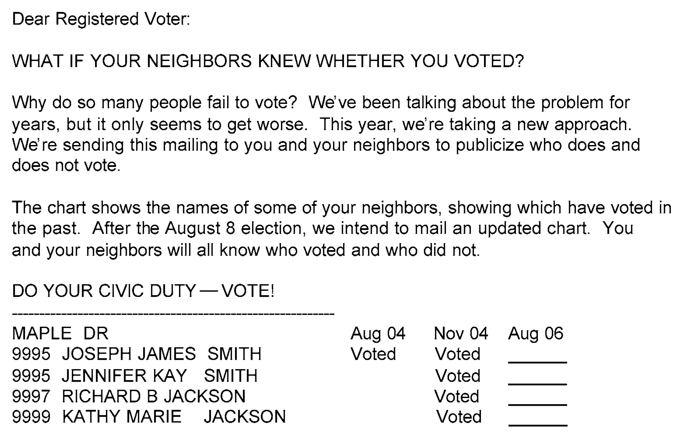
Causal effect of naming-and-shaming on turnout
Social Pressure Experiment [Optional]
August 2006 Primary Statewide Election in Michigan1
Send postcards with different (randomly assigned) messages
no message (control group)
civic duty message
“you are being studied” message (Hawthorne effect)
neighborhood social pressure message
1 Gerber, Alan S., Donald P. Green, and Christopher W. Larimer. 2008. "Social pressure and voter turnout: Evidence from a large-scale field experiment." American Political Science Review 102 (1): 33--48.
Analysis
Turnout by Group:
| Civic Duty | Control | Hawthorne | Neighbors |
|---|---|---|---|
| 0.31 | 0.3 | 0.32 | 0.38 |
SATE for each group:
| Civic Duty | Hawthorne | Neighbors |
|---|---|---|
| 0.02 | 0.03 | 0.08 |
- Randomization balances covariates across groups:
Primary 2004 for each group:
| Civic Duty | Control | Hawthorne | Neighbors |
|---|---|---|---|
| 0.4 | 0.4 | 0.4 | 0.41 |
Observational Studies
Often, we can’t randomize treatment for ethical and logistical reasons:
- e.g., smoking and lung cancer
Observational studies: naturally assigned treatment
Better external validity for generalization beyond experiment
Weaker internal validity:
pre-treatment variables may differ between treatment and control groups
confounding bias due to these differences
selection bias from self-selection into treatment
statistical control needed
unobserved confounding poses a threat
Confounding
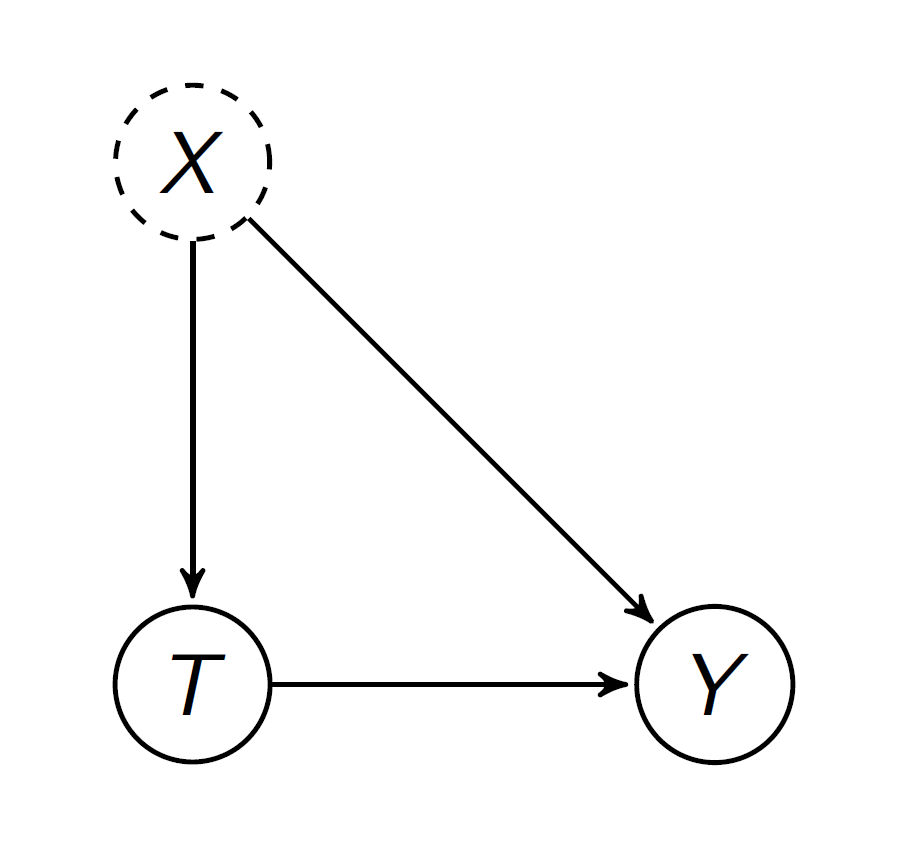
Key assumption “Unconfoundedness”: treatment and control groups comparable with respect to everything other than treatment
How can we find a good comparison group?
Asthma in Children [Optional]
New evidence for the role of microbes from farm animals in dust
Comparison of Amish and Hutterites:
similar genetic backgrounds, large families, and a simple communal life style
diets are similar, little exposure to tobacco or pollution, both groups prohibit indoor pets, meticulously clean homes
Rates of asthma in children: 2–4% (Amish) vs. 15–20% (Hutterites)
Findings:
Amish do not use electricity, but Hutterites do
Amish kids play in animal barns
Amish kids have better immune system, leading to less allergic reaction
Giving Amish house dust to mice protected them from allergens whereas Hutterites house dust did not
Minimum Wage and Unemployment
How does the increase in minimum wage affect employment?
Current debate: federal minimum wage increase
Many economists believe the effect is negative
especially for the poor
also for the whole economy
Hard to randomize the minimum wage increase
Two social scientists tested this using fast food chains in NJ and PA
In 1992, NJ minimum wage increased from $4.25 to $5.05
Neighboring PA stays at $4.25
Observe employment in both states before and after increase
NJ and (eastern) PA are similar
Why limit to fast food chains?
Fast food chains are the most affected by min wage
Did the Minimum Wage Law Affect the Wages in NJ?
Before
| > 5.05 | < 5.05 | |
|---|---|---|
| NJ | 0.09 | 0.91 |
| PA | 0.06 | 0.94 |
After
| > 5.05 | < 5.05 | |
|---|---|---|
| NJ | 0.997 | 0.003 |
| PA | 0.045 | 0.955 |
Are the NJ and PA Restaurants Comparable?
Average wages before the increase in minimum wage:
| NJ | PA |
|---|---|
| 4.61 | 4.65 |
Prior proportion of fulltime employment:
| x | |
|---|---|
| NJ | 0.297 |
| PA | 0.310 |
Cross-Section Comparison
Compare NJ and PA using the data after the increase
The treatment and control groups are assumed to be identical on average in terms of all confounders
What confounders are missing from the data?
Assumptions:
No cross-sectional contamination
No cross-sectional confounders
Compute the proportion of fulltime employees after the increase:
ˉY(1)−ˉY(0)=ˉY(NJafter)−ˉY(PAafter)=0.0481
Here, NJ (after the increase) is the treatment group and PA (after the increase in NJ) is the control group.
This is our estimated SATE. Why "estimated"?
The actual SATE is not observed due to the fundamental probelem of never observing the counter-factual.
Before and After Comparison
State-specific confounders for cross-section comparison
Compare NJ before and after
Assumptions:
No temporal contamination (treatment is exogenous)
No (temporal) confounders
What might be time-varying confounders?
ˉY(1)−ˉY(0)=ˉY(NJafter)−ˉY(NJbefore)=0.0239
- Here, NJ (after the increase) is the treatment group and NJ (before the increase) is the control group.
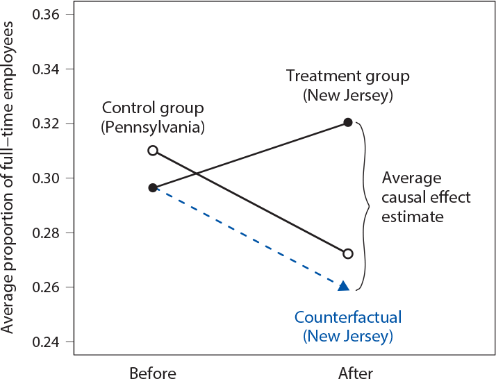
Difference-in-Difference
Key Idea: use PA before-and-after difference to figure out what would have happened in NJ without the increase
NJ before-and-after difference addresses within-state confounding
Assumptions:
Parallel time trends (how good is our control group)
Treatment is exogenous (no temporal or cross-sectional contamination)
Estimate the sample average treatment effect for the treated (SATT), NOT SATE
ˉY(NJafter)−ˉY(NJbefore)−(ˉY(PAafter)−ˉY(PAbefore))=0.0616
Visualizing Difference-in-Difference
The Difference-in-Difference Design
A natural experiment always has the control group (observations not affected by the change) and the treatment group (observations that are affected).
Need data for two time periods (before and after the treatment).
Thus, four groups of observations: control before, treatment before, control after, treatment after
The difference between the two before groups helps account for the differences between the treatment and control groups that are not caused by the treatment.
Summary of 3 Identification Strategies
Cross-section comparison
Compare treated units with control units after the treatment
Assumption: the treated and control units are comparable
Possible unit-specific confounding
Before-and-after comparison
Compare the same units before and after the treatment
Assumption: no time-varying confounding
Difference-in-Differences
Assumption: parallel time trend
Under this assumption, it accounts for both unit-specific and time-varying confounding
- None of the approaches is best. They require different assumptions.
Incinerator and Home Prices [Optional]
Suppose we would like to study the effect of proximity to a garbage incinerator on home prices.
Propose a cross-sectional natural experiment design to study this question. What is the key assumption for this design? Does it hold?
Propose a before-and-after comparison design to study this question. What is the key assumption for this design? Does it hold?
Propose a diff-in-diff design to study this question. What is the key assumption for this design? Does it hold?
Which of the proposed design would work the best in this example?
Lab Questions
Download and open the data on housing prices,
hprice3.Create a binary variable,
nearincthat equals to 1 if the house is within 3 miles of the incinerator.How many houses are there in the data in each year?
Compare the average house price in 1978 between the houses near and far from the incinerator.
Compare the average house price in 1981 between the houses near and far from the incinerator.
Implement the diff-in-diff design.